Skewness is one of the less-known but practical measures from statistics that can be used in trading. It is defined as a measure of the asymmetry of the probability distribution of a random variable around its mean. Financial mathematics and most quantitative models assume some kind of symmetric distribution of random variables, such as near-normal distribution, which would have zero skewness. From the perspective of traders, it is always interesting to look for extreme values of skewness which attributed to non-expected outcomes. When you bet a reasonable amount of capital on non-quite-probable but good-calculated events, it is possible to catch a chunk of those tails risks while also possible to hedge harmful exposure (if you have some of the opposite exposure). But is using skewness as a factor in a systematic strategy really profitable?
Video summary:
A plot of normal distribution (or bell-shaped curve) where each band has a width of 1 standard deviation, from Wikipedia.
The goal of this analysis is to explore the commodity skewness trading strategy and perform the battery of robustness tests to see how sensitivity analysis changes overall results regarding performance, volatility, and Sharpe ratios.
We have covered the topic of robustness testing topic extensively; we also mentioned the lottery effect and possible asymmetric payoffs that make skewness as a predictor an especially lucrative topic for trading strategies. We encourage you to look at similar of our past posts on our Blog.
Commodities are a specific type of asset class primarily consisting of physical goods. Commodity markets are often extremely volatile during geopolitical turmoil and economic uncertainty. Interestingly, while the stock (equity) market hates instability, and when it is not sure about the future prospects of Fed policy or companies’ earnings, it drops (into corrections, or even worse, bear markets); commodity markets love uncertainty and generally rise in case of an unclear and gloomily predicted future (bloom into bull markets). Therefore, the skewness strategy can be finely utilized as a hedge in case of significant exposure to publicly traded stocks worldwide. Exposure to commodities can be obtained by owning an ETF, but our study uses data from underlying rolled futures contracts. Futures are derivative auction markets in which participants (be it producers [hedgers], consumers, and speculators [traders]) buy and sell commodities and futures contracts for delivery on a specified future date.
Data
CME is the codename of the Chicago Mercantile Exchange, the leading world futures and options trading venue, and ICE is Intercontinental Exchange®. At the same time, the name of the commodity is encoded after the underscore, and in the second column is self-explanatory.
We use an updated data sample of 33 years, from early 1990 to nowadays. In total, we analyzed portfolio of 22 different commodities:
Symbol of Futures Continuous Contract
Commodity Name
CME_S1
Soybean Futures
CME_W1
Wheat
CME_SM1
Soybean Meal
CME_BO1
Soybean Oil
CME_C1
Corn
CME_O1
Oats
CME_LC1
Live Cattle
CME_FC1
Feeder Cattle
CME_LN1
Lean Hog
CME_GC1
Gold
CME_SI1
Silver
CME_PL1
Platinum
CME_CL1
Crude Oil
CME_HG1
Copper
CME_NG1
Natural Gas (Henry Hub) Physical
CME_PA1
Palladium
ICE_CC1
Cocoa
ICE_CT1
Cotton No. 2
ICE_KC1
Coffee C
ICE_O1
Heating Oil
ICE_OJ1
Orange Juice
ICE_SB1
Sugar No. 11
Model & Base Case Test
Trading Strategy
Each month investor calculates the skewness of each commodity. In our base case, we use daily data for a period of 12 months for calculation. The strategy deployed consists of an individual investor going long n commodities with the lowest skewness (negative skew) and shorting n commodities with the highest skewness (positive skew), where n range from 1 to 11. We assume each selected commodity future has an equal weight in the final portfolio, which is rebalanced periodically on a monthly basis. Our strategy follows, is built on, and is roughly inspired by strategy #281 Skewness Effect in Commodities and blog Skewness / Lottery Effect in Commodities.
The picture from Wikipedia visually explains different skewed distributions and depicts that the mean and the median have different relationships in them.
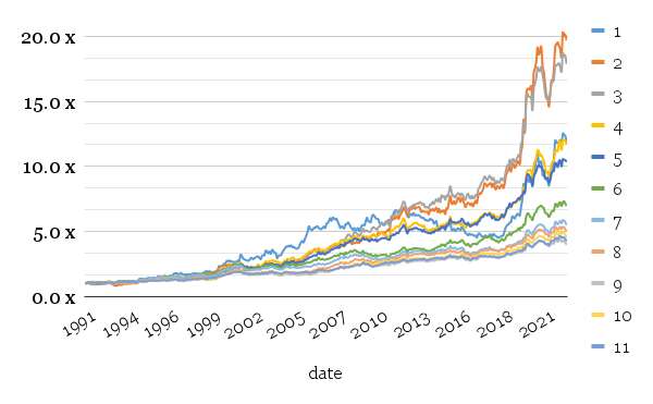
We will always analyze 3 variants of the Skewness strategy: long-short, long-only, and short-only portfolios. Let’s take a look at results from a long-short portfolio of buying and selling x/x number of commodity contracts simultaneously. Y-axis always shows total appreciation of the sum devoted to the exact one x/x version of the strategy.
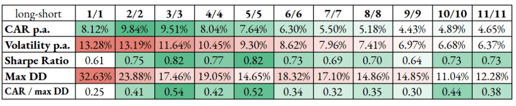
Long-short variant:
This is a standard application of the skewness approach; it smooths the overall equity curve, lowering drawdowns and volatility. Exposure to a modest (3-6) number of commodities also provides the sweet spot for PMs trying to optimize Sharpe ratios. Best returns are achieved using a strategy going long and simultaneously short the worst and the best 2 commodities.
As we will see further from comparing with other long-only and short-only models, a more diversified model of going both long and short the best and the worst commodities hurts overall performance but significantly dampens volatility and maximal drawdown.
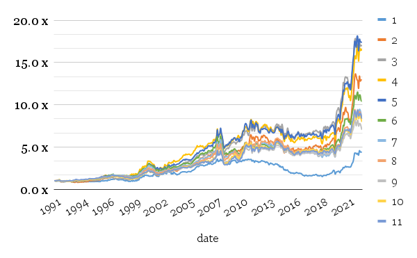
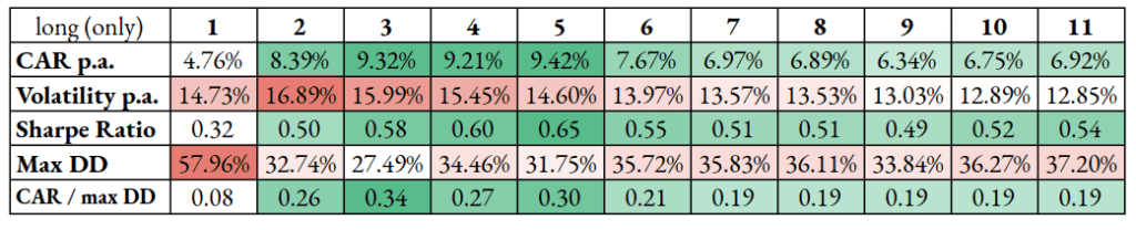
Long only variant:
For long legs only, volatility is significantly increased when not having a diversified basket of commodities in a long-only portfolio. Maximum drawdown is also elevated. Compared to the long-short strategy, this variant, with all types of its variations, provides excellent returns for speculators but significant volatility.
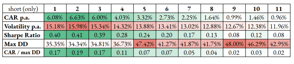
Short-only variant:
In 2022, the strategy worked as an excellent hedge against geopolitical tensions. Furthermore, an exceptional strategy success attribute was negative crude oil future prices for a short time span during the Covid outbreak in 2020. Aggressive concentrated exposure (less than 3 commodities), according to skewness in short legs, provides the optimal strategy for mitigating risk or enriching your diversification if you have mostly equity exposure.
It is generally worth shorting fewer commodities simultaneously based on skewness alone for purely performance purposes. However, volatility in the case of selling commodities alone is still extreme, and some of the drawdowns are also brutal.
Model Expansion & Robustness Tests
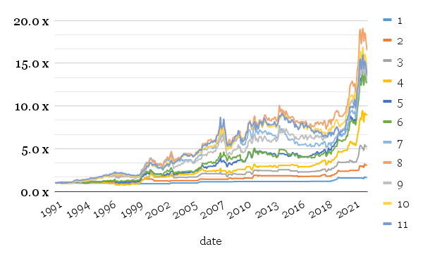
Momentum in commodities, and eventually, all markets, is a well-known concept and often the cornerstone of trend-following. It is an interesting application to combine it with skewness to enjoy both advantages and minimize drawdowns possibly. Or not? Our idea was to combine the most used factor in commodities, momentum, with an experimental approach of skewness. We tried to merge both approaches and here are the results…
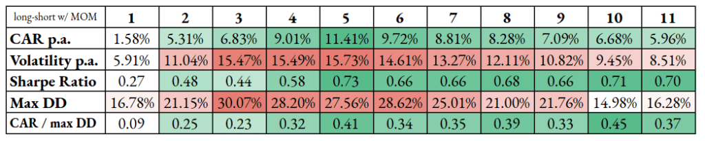
The combination of skewness with momentum uses logical AND rule. In the case of momentum, we are long n number of best-performing assets and, at the same time, short the same number of commodity futures. In the case of skewness, we are long n number of assets with the lowest skewness and, at the same time, short the same number of commodity futures with the highest skewness. Now, both conditions must be fulfilled if the commodity is to be included in the model. Therefore, it must be among the best in momentum and among the lowest skewed for a long position (and vice versa for a short position).
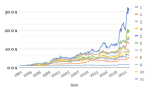
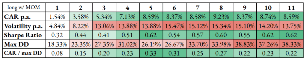
Long-short variant:
Compared to our basis case, i.e., skewness without momentum, the long-short model with momentum provides us with improved returns with higher volatility in the case of more than 4 assets. Especially 5/5 model is exceptional, but the disadvantage is really higher volatility. So Sharpe ratios, overall, are hurt.
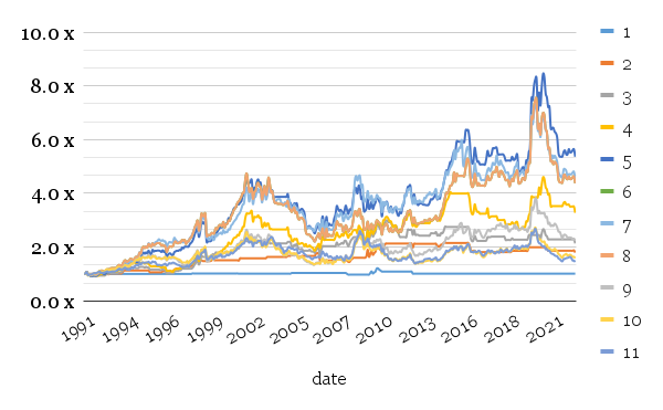
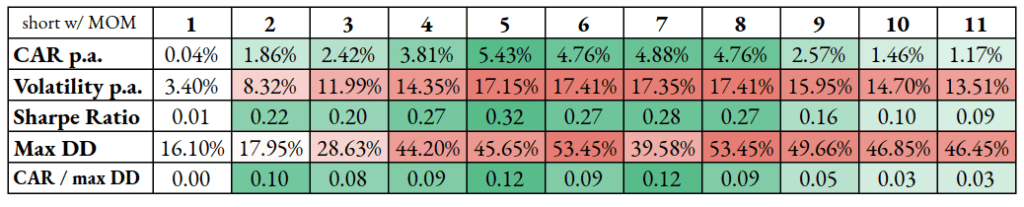
Long only variant:
When considering the long-only model adjusted by the momentum component, the best results are achieved by selecting 8 commodities. Again, higher volatilities and high drawdowns might be problematic in systematic portfolios or strict trend-followers.
Compared with our base case scenario (skewness only), momentum adds no considerable value to performance or volatility dampening. While returns in both applications (without and with momentum) stay roughly the same (with momentum factor smoothing them over a larger number of commodities), volatility is even worse here.
Short-only variant:
Finally, for short-only variants, the momentum does not add any advantage to the short-only skewness model.
Short conclusion:
Unfortunately, we have to refute our hypothesis that a double sort of skewness with momentum would provide investors with significant benefits, so we would advise using a single sort of skewness alone.
Variable Initial Period
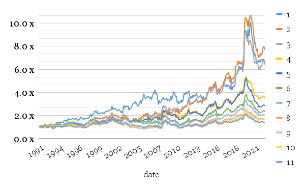
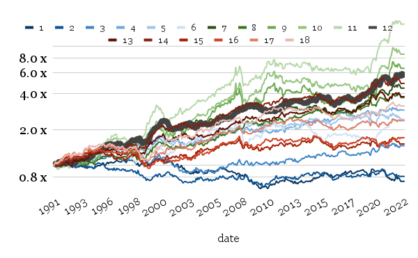
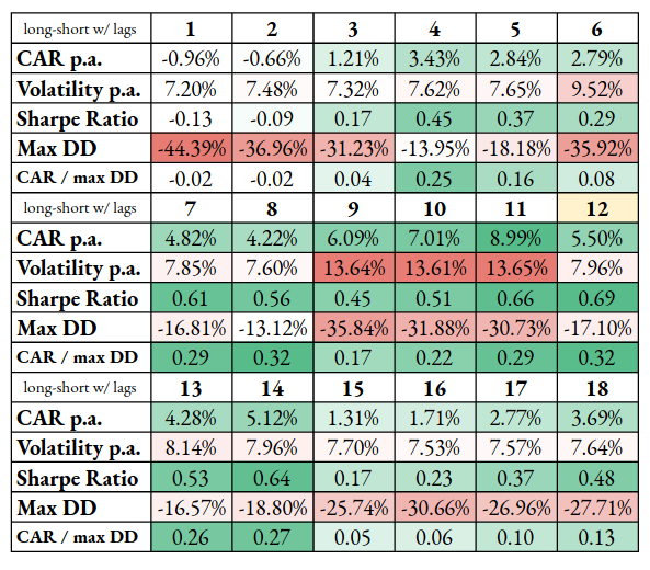
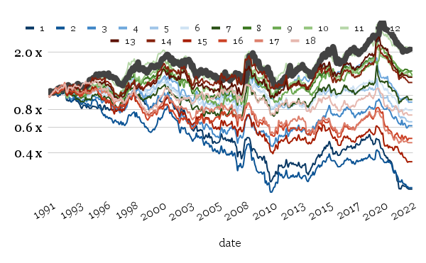
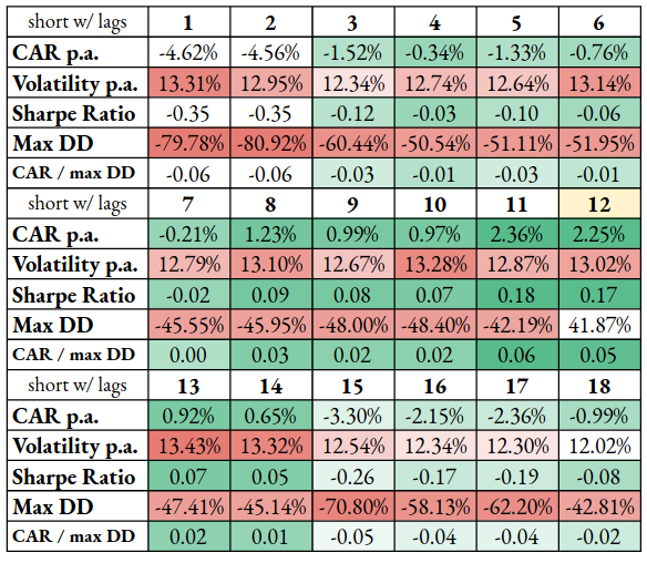
In this battery of robustness tests, the calculation period for the skewness (originally fixed to 12 months) is now varying, from 1 month to 18 months (the step is always one month). We always use the 7/7 variant of the commodity skewness model (going long 7 commodities with the lowest skewness and going short 7 commodities with the highest skewness).
We now introduce of use of log y-scale to better depict the overall performance of the portfolios. A base case of 12 months is highlighted with a strong black line in the graph and a light yellow background in the table. For lower time-lag months, we use shades of blue, mid-interval, green, and higher-than-base red.
Long-short variant:
In the case of the long-short portfolio with varying initial periods, we do not gain any significant outperformance against the base 12-month calculation period case, except for the 9, 10, 11 months calculation period. Overall, all calculation periods for skewness between 7 and 14 months look satisfactory.
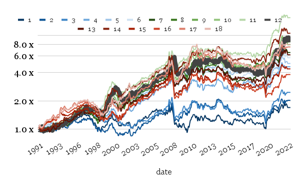
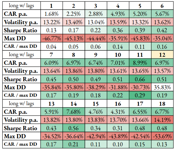
Long only variant:
The long-only portfolio variants again look satisfactory for the calculation periods from 7 till 14 months. With expanding (or decreasing) time horizon of an initial period, both the volatility and drawdowns rise significantly.
Short-only variant:
The short-only variants are the most troublesome. The 12-month calculation period is the best performing, and performance (and Sharpe ratios) significantly decreases if we deviate in each direction from the base case variant too much.
Short Conclusion
The goal of the article was to run a battery of robustness tests to evaluate the base (12-month) variant of the skewness strategy on commodities. What’s the conclusion? As we have shown, a significant part of the performance and Sharpe ratio are retained in most of the strategy’s tested sub-variants. In most cases, when we change the strategy’s parameter (be it the skewness calculation period, the number of selected assets, or if we drop the long or short leg from the strategy), the strategy still performs satisfactorily.
We also tried to combine the skewness strategy with the commodity momentum. Although we hoped for further improvement of the strategy, unfortunately, double-sorted variants with momentum do not offer any advantage against the base case. Therefore, it probably doesn’t make sense to complicate the strategy with the usage of an additional momentum factor.
Just a side final note on strategy’s implementation: Our model uses data on commodity futures. The strategy may be replicated using ETFs with some tracking error (as there are some commodities that are not tracked by ETFs, therefore, we have a smaller investment universe) or even CFDs in case of favorable tax/overnight margin treatment.
Quantpedia is The Encyclopedia of Quantitative Trading Strategies
We’ve already analysed tens of thousands of financial research papers and identified more than 700 attractive trading systems together with hundreds of related academic papers.
This website uses cookies so that we can provide you with the best user experience possible. Cookie information is stored in your browser and performs functions such as recognising you when you return to our website and helping our team to understand which sections of the website you find most interesting and useful.
Strictly Necessary Cookies
Strictly Necessary Cookie should be enabled at all times so that we can save your preferences for cookie settings.
If you disable this cookie, we will not be able to save your preferences. This means that every time you visit this website you will need to enable or disable cookies again.